Model Predictive Control
(maybe AI generated (but checked I swear :pray: :pray: :pray:))
1. The Core Philosophy: “Look Ahead, Act Now”
Model Predictive Control (MPC) is not just a control law; it is an optimization strategy that runs in real-time. Unlike traditional controllers (like PID) that react primarily to past errors, MPC is proactive.
As described in the lecture notes, MPC operates like a chess player:
- Prediction: The player projects the game scenario into the future to predict how the opponent will respond to a sequence of moves.
- Optimization: They choose the best sequence of moves to maximize their chances of winning.
- Receding Horizon: If the opponent replies unexpectedly, the player doesn’t stick to the old plan. They reschedule the strategy based on the new situation.
2. How does it work?
At every single sampling instant $k$, the MPC controller performs a complex cycle of operations. Here is the step-by-step breakdown:
Step 1: Measurement and State Estimation
The controller reads the current state of the plant, $x(k)$. If the state cannot be fully measured, an estimator (like a Kalman Filter) is used to reconstruct it.
Step 2: Prediction (The Internal Simulation)
Using the dynamic model of the plant, $x(k+1) = Ax(k) + Bu(k)$, the controller simulates the future behavior of the system over a specific window called the Prediction Horizon ($H_p$).
Step 3: Solving the Optimization Problem (QP)
The controller must find a sequence of future control inputs $U(k) = [u(k|k), \dots, u(k+H_p-1|k)]$ that minimizes a cost function $J$. This is typically solved as a Quadratic Programming (QP) problem.
The cost function generally looks like this: \(J = \sum_{i=0}^{H_p-1} \left( x^T(k+i|k)Qx(k+i|k) + u^T(k+i|k)Ru(k+i|k) \right) + x^T(k+H_p|k)Sx(k+H_p|k)\)
The “Tuning Knobs” Explained:
- $Q$ (Performance): Penalizes the state error. A high $Q$ forces the system to reach the setpoint quickly.
- $R$ (Control Effort): Penalizes the use of actuator energy. A high $R$ makes the controller “gentle” and smooth.
- $S$ (Terminal Weight): Penalizes the final state at the end of the horizon ($H_p$). This is crucial for mathematical stability, ensuring the system doesn’t drift away after the prediction ends.
Step 4: Handling Constraints
Unlike other controllers, MPC explicitly considers physical limitations during the calculation. It ensures the solution satisfies:
- Input Constraints: e.g., $-1 \le u(k) \le 1$. This represents physical limits like valve saturation or maximum voltage.
- State Constraints: e.g., $x_{min} \le x(k) \le x_{max}$. This ensures safety (e.g., keeping temperature below a critical limit).
Step 5: The “Receding Horizon” Action
Once the optimal sequence $U^*$ is found, the controller applies only the first element $u(k) = u^*(k|k)$ to the real system. The rest of the computed sequence is discarded. At the next time step ($k+1$), the entire process starts over with fresh measurements. This feedback loop allows the controller to correct for model inaccuracies and external disturbances.
3. Advanced Mechanics: Managing Complexity
Prediction Horizon ($H_p$) vs. Control Horizon ($H_c$)
Calculating a unique control input for every step of a long prediction horizon can be computationally expensive (we’ll have more degrees of freedom $\Rightarrow$ more complex). To solve this, MPC separates the horizons:
- Prediction Horizon ($H_p$): How far we “see” into the future.
- Control Horizon ($H_c$): The number of steps we are allowed to change the control input, where typically $H_c \le H_p$.
The Strategy: After the first $H_c$ steps, the control signal is often held constant or forced to follow a specific law for the remainder of the prediction window ($H_p - H_c$). This reduces the degrees of freedom in the optimization, making the calculation faster without significantly hurting performance.
[### What are the possible solutions? One possible solution is to “see more than what we optimize”. What does it mean? We predict system behaviour over the finite horizon $H_p$, but we optimize only the first $H_c \leq H_p$ steps. The remaining control values can be set in different ways.
Another possibility is variable blocking: control moves are grouped so that their value is “blocked” for 2 or more prediction steps.
Last one is useful is we have system delays or “inverse response”. In this case, instead of optimize every states, we focus on the states only after the delay or the inverse response.]: #
4. Output tracking
We can include output tracking, by adding in the cost function a quadratic term of the form
\[(y(k+i \mid k)-r(i))^T \ Q\_y \ (y(k+i \mid k) - r(i))\]as we can see, this quadratic term depends on the quantity $(y-r)$.
[!IMPORTANT] Output constraints can be included too! These constraints are translated in linear inequalities in $U(k)$, similar to what we saw for $u$ and $x$ constraints
Handling steady-state tracking error
A standard state-space MPC regulates states to zero. To track a non-zero reference $r(k)$ without steady-state tracking error (i.e. $e_r^\infty = 0$), we must introduce Integral Action.
In MPC, this is done by changing the optimization variable from the absolute input $u(k)$ to the input increment $\Delta u(k)$:
\[\Delta u(k) = u(k) - u(k-1)\]Why does this work?
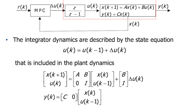
- Mathematical Integrator: By using $\Delta u$, we effectively insert a discrete-time integrator $\frac{z}{z-1}$ into the control loop. In fact, in z domain, we have $U(z) = \frac{z}{z-1}\Delta U(z)$ and this is a discrete time integrator.
- Augmented State: The system model is “augmented” (expanded) to include the previous input as part of the state vector:
[!NOTE] The second equation comes from $u(k) = u(k-1) + \Delta u(k)$ (basically it’s just the input increment $\Delta u(k)$ equation expliciting $u(k)$.)
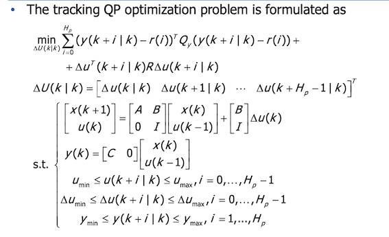
The cost function then minimizes the error between the output and the reference $(y - r)$, as well as the control changes $\Delta u$. This guarantees that when the system settles (steady state), the error is zero!
The final system, with its matrix equations, optimization problem and constraints is shown below:
MPCtools
see live script on exercise folder