LQR: Linear-Quadratic Regulator
1. Fundamentals of Optimal Control (LQR)
The Need for Optimal Control: Beyond Pole Placement
The Linear-Quadratic Regulator (LQR) design method emerges as a foundational solution, particularly when control requirements cannot be defined simply by specifying the desired closed-loop pole locations, which is the core of the classical Pole Placement (PP) method.
Dynamic systems often feature conflicting performance objectives that don’t translate neatly into transient response constraints, but rather into a structured trade-off. A motivating example is active suspension control in vehicles. Achieving maximum comfort requires “soft” suspensions to isolate from road solicitations, while maximizing handling (tire-road contact) requires a “stiffer” structure. These objectives are inherently antagonistic, and the control problem is reduced to finding the optimal balance, formalized through mathematics, rather than pre-defining specific pole locations.
The LQR, an optimization-based approach, overcomes a key limitation of purely deterministic methods like PP. In multi-input, multi-output (MIMO) or high-order systems, choosing all desired pole locations arbitrarily can be extremely complex and fails to explicitly account for the energy or control effort required to achieve them.
2. Continuous time LQR
We start our analysis from the continuous time LQR. Let’s assume a static state feedback architecture $u(t) = - k x(t)$. The continuous time LQR problem eeks the control law $u(t)$ that minimizes the objective function $J(u)$
The Weighting Matrices
- State Weighting Matrix ($Q$): $Q \in \mathbb{R}^{n,n}$, symmetric and positive semi-definite ($Q = Q^{\top} \ge 0$). It penalizes the deviation of the state $x(t)$ from zero. Increasing $Q$ makes state deviation “costly,” forcing a more aggressive response.
- Control Weighting Matrix ($R$): $R \in \mathbb{R}^{p,p}$, symmetric and positive definite ($R = R^{\top} > 0$). It penalizes the magnitude or energy of the control signal $u(t)$. Increasing $R$ makes control effort “costly,” forcing a more conservative response.
The Algebraic Riccati Equation (ARE) and Optimal Gain $K$
The optimal solution $u(t)$ is given by $u(t) = -Kx(t)$.
The optimal gain $K$ is computed using the unique, positive definite solution $P$ to the Algebraic Riccati Equation (ARE).
Algebraic Riccati Equation (ARE):
The Optimal Gain $K$ is then calculated directly from $P$:
\[K = R^{-1}B^{T}P \in \mathbb{R}^{p,n}\]\[M_{R}(A,B)=\begin{bmatrix} B & AB & \cdots & A^{n-1}B \end{bmatrix}\]💡 Intuition Check: The Role of P : The matrix $P$ isn’t just an arbitrary variable; it represents the minimum total cost remaining (or “cost-to-go”) from the current time to infinity, given the current state $x(t)$. The calculation of $K$ naturally emerges from minimizing this cost.
Existence, Stability, and Structural Prerequisites
The stability and existence of the LQR solution depend critically on the underlying structural properties of the system matrices.
Guaranteed Asymptotic Stability
The LQR control law $u(t)=-Kx(t)$ guarantees that the closed-loop system $\dot{x}(t)=(A-BK)x(t)$ is asymptotically stable, provided two structural conditions are met:
Condition: The rank of $M_{R}$ must equal the state dimension $n$: $\rho(M_{R}) = n$.
Observability of the Penalized States
Asymptotic stability is guaranteed if the pair $(A, C_q)$ is observable, where $C_q$ is defined such that $Q = C_{q}^{T}C_{q}$.
The Observability Matrix $M_O(A,C_q)$ must have full rank
Condition: The rank of $M_{O}(A,C_q)$ must equal $n$: $\rho(M_{O}(A,C_q)) = n$.
⚠️ Critical Warning on Stability
If an unstable mode exists in the system but is not “observed” (i.e., not penalized) by the weighting matrix $Q$, the LQR algorithm has no incentive to stabilize it. This condition is why observing the penalized states (via $C_q$) is crucial for stability guarantees.
3. Discrete-Time LQR (DLQR) and Digital Implementation
For real-world implementation on digital processors, the continuous system must be discretized, leading to the Discrete-Time LQR (DLQR) problem.
4.1 The DLQR Formulation
The discrete LTI system dynamics are represented by $x(k+1) = A x(k) + B u(k)$.
The DLQR problem minimizes the cost function expressed as a summation over the infinite horizon:
where $A$ and $B$ are the discrete state-space matrices, and $Q_D$ and $R_D$ are the discrete weighting matrices. The optimal control law is $u^{*}(k) = -K_D x(k)$.
4.2 The Discrete Algebraic Riccati Equation (DARE)
The optimal gain $K_D$ depends on the matrix $P$ that solves the Discrete Algebraic Riccati Equation (DARE):
\[P = A^T P A - A^T P B (B^T P B + R_D)^{-1} B^T P A + Q_D\]The Optimal Gain $K_D$ is calculated as:
\[K_D = (B^T P B + R_D)^{-1} B^T P A\]4.3 Practical Tuning: The Intuitive Power of Q and R Tuning
Q and R is the engineering art of LQR design. It involves finding the ratio that delivers acceptable performance (transient response, speed, damping) while respecting actuator limits.
The Trade-Off Guide:
| Goal | Action | Effect |
|---|---|---|
| Faster Response / Better Regulation | Increase values in Q relative to R. | The resulting gain K increases, leading to a more aggressive controller and faster pole locations (closer to the origin in the z-plane). |
| Increased Damping / Reduced Overshoot | Increase the penalty on the velocity/rate states (e.g., x-dot) within the Q matrix. | The controller reduces the use of energy that would induce excessive velocity, increasing the effective damping ratio (zeta). |
| Reduced Control Effort / Lower Energy Use | Increase values in R relative to Q. | The resulting gain K decreases, leading to a more conservative controller. The system response slows down, and states may deviate more from zero. |
LQR with setpoint tracking
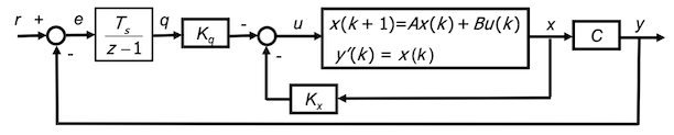
A reference “input” can be included as shown:
![]()
As seen in 1 DoF architecture, we are interested in limiting tracking error $e(k)$, that is the defined as $e(k) = y(k)-r(k)$. So, zero steady state tracking error $e_{inf}$ can be achieved by introducing the DT “integral” $q(k)$ of the tracking error $e(k)$ as an additional system state
\[q(k+1) = q(k) + T_s(r(k)-y(k)) q(k) + T_se(k)\]What is the meaning of $q(k+1)$ if we divide by $T_s$?
In the left hand side we obtain the incremental ratio (ie the derivative!). Since $q$ is the integral of $e$ $\Rightarrow$ $e$ is the derivative of $q$!
We have a richer control architecture than on a side it’s the same contribution already analysed and on the other side an extra blocks referred to tracking error.
The state feedback control architecture is modified as shown below
We’ll see that in stability condition, the tracking error $e(k)$ is 0!
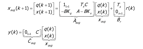
Without loss of generality, we consider the SISO case. Let’s consider the augmented state that includes the time integral of the tracking error:
\[X_{aug}(k) = \begin{bmatrix} q(k) \\ x(k) \end{bmatrix} \in \mathbb{R}^{n+1}, q(k) \in \mathbb{R}\]→ The corresponding state equation is:
It can be proved that the system guarantees zero steady state tracking error when the reference signal r is constant!
The design of the LQR control law with the integral state is performed using as system matrices $A_{aug}$ and $B_{aug}$.
To simplify our analysis, let’s introduce also this property:
if the couple $(A,B)$ is reachable, then also $(A_{aug},B_{aug})$ is reachable!