Constraints handling in control design
Physical limitations of the actuator device impose hard constraints on the control input $u(t)$. For example, a possible constraint can be a saturation constraint of the form
\(-u_M \leq u(t) \leq u_{M}, \, \forall t \geq 0\)
\(\Rightarrow |u(t)| \leq u_{M}, \, \forall t \geq 0\)
The saturation constraint can be described as a nonlinear static function of the control input as
$m(t)$ → saturated input
Note that, when $-u_M \leq u(t) \leq u_M \Rightarrow m(t) = u(t)$
When the input saturation is active (i.e. when either $u(t) > u_M$ or $u(t) < - u_M$), the feedback control system is non-linear.
In the presence of saturation, control system work without feedback $\Rightarrow$ exceeding the input prescribed bounds leads to unexpected system behaviours such as large overshoots, low performace, or, in the worst case, instability🙀
How we can handle this situation?
Input saturation constraint cannot be handled directly by neither pole placement nor optimal control design procedures, but it must be checked a posteriori through simulation.
If such a requirement is not met, a common procedure is to slow down the transient response of the control system, e.g., by choosing dominant closed loop poles with larger time constants.
However, an increase of the closed loop dominant time constant may cause a degradation of the transient performance (i.e., rise time and settling time) → conflicting requirements.
Approches to constrained control
- Caution → back off performance demands so constraints are met → slow down the controller
- Serendipitous → allow occasional constraint violation (i.e. saturate the control input without modifying the original design) → used if the difference between input and saturation is small
- Evolutionary → begin with a linear design and add embellishments, for example, anti-windup → build an additional structure to handle saturation
- Tactical → include constraints from the beginning, for example, Model Predictive Control
Finite horizon constrained control
Analytic formulation without constraints (see ex1 in matlab)
We need both discrete time approach and optimal control, since in discrete time we can handle the situation in discrete time instant (easier than in continuous time).
Let’s consider discrete time, finite horizon, linear quadratic optimal control.
First of all, we consider the solution in the absence of input constraints.
For an LTI discrete-time dynamical systems described by the state equation
At the generic time instant $k$, the finite horizon (Linear Quadratic) optimal control is formulated as
\[\min_{U(k)} J(x(k), U(k)) = \min_{U(k)} \left[ \sum_{i=0}^{H_p-1} \left( x(k+i)^\top Q x(k+i) + u(k+i)^\top R u(k+i) \right) + x(k+H_p)^\top S x(k+H_p) \right]\]Let’s define
\[U(k) = \begin{bmatrix} u(k) & u(k+1) & \dots & u(k+H_p-1) \end{bmatrix}\]with $H_p \to$ time prediction horizon
In discrete time, the unconstrained optimal solution $U^*(k)$ can be easily computed through a finite dimensional quadratic optimization problem (slides L08_15-21). Let’s consider $H_p = 3$ → our aim is to compute the sequence $U(k) = [u(k) \ \ u(k+1) \ \ u(k+2)]$ → we express the function as a function of $U(k)$ and the initial state $x(k)$
\[\mathcal{A} = \begin{bmatrix} A \\ A^2 \\ A^3 \end{bmatrix}\][!WARNING] The computation of the cost function is omitted, see slides
New matrices notation
Before defining the cost function and find the optimal input $U^*(t)$, we need to define the new system matrices that we will use (remember that $H_p = 3$)
\(\mathcal{B} = \begin{bmatrix} \quad B \quad 0_{px1} \quad 0_{px1} \\ AB \quad B \quad 0_{px1} \\ A^2B \quad AB \quad B \\ \end{bmatrix}\) \(\mathcal{Q} = \begin{bmatrix} \quad Q \quad \ 0_{nx1} \quad 0_{nx1} \\ 0_{nx1} \quad \ Q \quad 0_{nx1} \\ 0_{nx1} \quad 0_{nx1} \quad S \\ \end{bmatrix}\) \(\mathcal{R} = \begin{bmatrix} \quad R \quad \ 0_{px1} \quad 0_{px1} \\ 0_{px1} \quad \ R \quad 0_{px1} \\ 0_{px1} \quad 0_{px1} \quad R \\ \end{bmatrix}\)
[!CAUTION] This matrices reported here refer to our example with $H_p = 3$! If $H_p \neq 3$ matrices dimensions are different!!!
At this point, we are almost done. We now define our cost function $J$ as
\[J(x(k), U(k)) = x^T(k)\mathcal{A}^T \mathcal{QA}x(k) + 2x^T(k)\mathcal{A}^T \mathcal{QB}U(k) + U^T(k)(\mathcal{B}^T \mathcal{QB} + \mathcal{R})U(k)\]And posing
\[H = 2(B^T \mathcal{QB} + \mathcal{R})\] \[F = 2\mathcal{A}^T \mathcal{QB}\] \[\overline{J} = x^T(k)\mathcal{A}^T \mathcal{QA}x(k)\]The cost function can be rewritten as
\[J(x(k), U(k)) = \frac{1}{2} U(k)^T HU(k) + x(k)^T FU(k) + \overline{J}\]→ which is quadratic in $U(k)$!
[!IMPORTANT] $H > 0$ is the Hessian matrix of the quadratic form $\Rightarrow$ it must be symmetric and positive definite. Why? Because we want a convex (local minimum = global minimum) cost function $\Rightarrow$ it must be positive definite!
So, given the quadratic form of the cost function, the solution can be computed in closed form as
\[U(k) = U^*(k) = - H^{-1}F^Tx(k)\]and in particular
\[U^{\ast}(k) = \begin{bmatrix} u^{\ast}(k) \\ u^{\ast}(k+1) \\ u^{\ast}(k+2) \end{bmatrix} = - H^{-1}F^Tx(k)\][!NOTE]
- the control sequence above is defined only over the considered time horizon (i.e. for $k \in [0, H_p-1]$ and can’t be extended to $k>H_p-1$ (in fact, in the considered example we have $H_p=3$))
- the optimal input at the generic time $k+i$ depends on the “ $i^{th}$ step ahead prediction” $x(k+i)$ of the state obtained by using the state space model and starting from the “initial condition” $x(k)$
[!IMPORTANT] We obtained that the optimal input sequence depends only on the measured state $x(k)$ and not on the present state $x(k+i)$
At this point we can easily compute ahead prediction of the state $X(k)$ as
\[X(k) = \mathcal{A}x(k) + \mathcal{B}U(k)\]As previously said, $X(k)$ depends only on $x(k)$!
“Analytic” formulation with constraints (see ex2 in matlab)
In this case, we will focus more on the intuitive understanding of the problem, instead of deriving analytic solution.
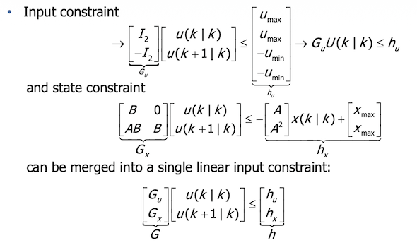
Our interest is including saturation constraints expressed as linear inequalities. As we can guess, we can have input saturation constraints, state saturation constraints or even both!
Let’s recall that when we are speaking about saturation constraints, we are meaning that
and the same for the state $x(k)$.
All linear inequalities are in $U(k)$ and can be recollected as follows:
Now we can optimize the quadratic function in the presence of linear constraints (quadratic programming). In order to do this, we use Matlab function quadprog() that computes optimal input $U^*(k)$.
[!NOTE] We don’t care about how does it work, we just need to define our matrices and our constraints. Matlab does the remaining part of the job. However, if you are really interested in what Matlab does, check this: Matlab-quadprog-docs
[!CAUTION] $U^(k)$ can be applied over the time horizon of length $H_p$ in open loop without any feedback. This makes weak the application of such a constrained finite horizon optimal control strategy in the presence of disturbances, uncertainty and measurement errors.
$\Rightarrow$ Feedback can be introduced by solving the considered constrained finite horizon optimal control at each time instant k by exploiting by the *Receding Horizon (RH) principle.
Receding Horizon principle
The RH principle is defined by the recursive procedure below.
At sample instant k:
- get the state $x(k) = x(k \lvert k)$
- solve the considered QP optimization problem w.r.t. $U(k \lvert k)$
- compute the minimizer $U^*(k \lvert k)$
- apply, as present control action, $u(k) = u^* (k \lvert k)$
- k← k + 1 and repeat the procedure
[!NOTE] If the model and the cost function are time invariant, the RH principle implicitly defines a nonlinear time invariant static state feedback control law of the form $u(k) = \mathcal{K} (x(k))$. However, the analytic expression of $\mathcal{K} (x(k))$ can’t be computed. It is possible to use RH principle also in finite horizon LQ unconstrained control, in order to obtain a feedback controller